Rotation formalisms in three dimensions

From Wikipedia, the free encyclopedia

(Redirected from Attitude representations)

Jump to: navigation, search

In geometry, various formalisms exist to express a rotation in three dimensions as a mathematical transformation. In physics, this concept extends to classical mechanics where rotational (or angular) kinematics is the science of describing with numbers the purely rotational motion of an object. The orientation of an object at a given instant is described with the same tools, as it is defined as an imaginary rotation from a reference placement in space, rather than an actually observed rotation from a previous placement in space.
According to Euler's rotation theorem the general displacement of a rigid body (or three-dimensional coordinate system) with one point fixed is described by a single rotation about some axis. Such a rotation may be uniquely described by a minimum of three parameters. However, for various reasons, there are several ways to represent it. Many of these representations use more than the necessary minimum of three parameters, although each of them still has only three degrees of freedom.
An example where rotation representation is used is in computer vision, where an automated observer needs to track a target. Let's consider a rigid body, with three orthogonal unit vectors fixed to its body (representing the three axes of the object's local coordinate system). The basic problem is to specify the orientation of these three unit vectors, and hence the rigid body, with respect to the observer's coordinate system, regarded as a reference placement in space.

Formalism alternatives

Rotation matrix

Main article: Rotation matrix

The above mentioned triad of unit vectors is also called a basis. Specifying the coordinates (scalar components) of this basis in its current (rotated) position, in terms of the reference (non-rotated) coordinate axes, will completely describe the rotation. The three unit vectors $\scriptstyle \hat{\mathbf{u}}$ , $\scriptstyle \hat{\mathbf{v}}$ and $\scriptstyle \hat{\mathbf{w}}$ which form the rotated basis each consist of 3 coordinates, yielding a total of 9 parameters. These parameters can be written as the elements of a 3 × 3 matrix $\scriptstyle \mathbf{A}$ , called a rotation matrix. Typically, the coordinates of each of these vectors are arranged along a column of the matrix (however, beware that an alternative definition of rotation matrix exists and is widely used, where the vectors coordinates defined above are arranged by rows^[1])

$\mathbf{A} = \left[ {\begin{array}{ccc} \hat{\mathbf{u}}_x & \hat{\mathbf{v}}_x & \hat{\mathbf{w}}_x \\ \hat{\mathbf{u}}_y & \hat{\mathbf{v}}_y & \hat{\mathbf{w}}_y \\ \hat{\mathbf{u}}_z & \hat{\mathbf{v}}_z & \hat{\mathbf{w}}_z \\ \end{array}} \right]$

The elements of the rotation matrix are not all independent—as Euler's rotation theorem dictates, the rotation matrix has only three degrees of freedom. The rotation matrix has the following properties:

A is a real, orthogonal matrix, hence each of its rows or columns represents a unit vector.
The eigenvalues of A are

$\{1, e^{\pm i\theta} \} = \{1,\ \cos(\theta)+i\sin(\theta),\ \cos(\theta)-i\sin(\theta)\}$

where i is the standard imaginary unit with the property i² = −1

The determinant of A is +1, equivalent to the product of its eigenvalues.
The trace of A is $\scriptstyle 1 \,+\, 2\cos(\theta)$ , equivalent to the sum of its eigenvalues.

The angle $\scriptstyle \theta$ which appears in the eigenvalue expression corresponds to the angle of the Euler axis and angle representation. The eigenvector corresponding with the eigenvalue of 1 is the accompanying Euler axis, since the axis is the only (nonzero) vector which remains unchanged by left-multiplying (rotating) it with the rotation matrix.
The above properties are equivalent to:

$\begin{align} |\hat{\mathbf u}| = |\hat{\mathbf v}| &= 1\\ \hat{\mathbf u} \cdot \hat{\mathbf v} &= 0\\ \hat{\mathbf u} \times \hat{\mathbf v} &= \hat{\mathbf w} \end{align}$

which is another way of stating that $\scriptstyle \hat{\mathbf u},\, \hat{\mathbf v},\, \hat{\mathbf w}$ form a 3D orthonormal basis. Note that the statements above constitute a total of 6 conditions (the cross product contains 3), leaving the rotation matrix with just 3 degrees of freedom as required.
Two successive rotations represented by matrices $\scriptstyle \mathbf{A}_1$ and $\scriptstyle \mathbf{A}_2$ are easily combined as follows: $\scriptstyle \mathbf{A}_\text{total} \;=\; \mathbf{A}_2\mathbf{A}_1$ (Note the order, since the vector being rotated is multiplied from the right). The ease by which vectors can be rotated using a rotation matrix, as well as the ease of combining successive rotations, make the rotation matrix a very useful and popular way to represent rotations, even though it is less concise than other representations.

Euler axis and angle (rotation vector)

A visualization of a rotation represented by an Euler axis and angle.

Main article: Axis angle

From Euler's rotation theorem we know that any rotation can be expressed as a single rotation about some axis. The axis is the unit vector (unique except for sign) which remains unchanged by the rotation. The magnitude of the angle is also unique, with its sign being determined by the sign of the rotation axis.
The axis can be represented as a three-dimensional unit vector $\scriptstyle \hat{\mathbf{e}} \;=\; [e_x\ e_y\ e_z]^\mathrm{T}$ , and the angle by a scalar $\scriptstyle \theta$ .
Since the axis is normalized, it has only two degrees of freedom. The angle adds the third degree of freedom to this rotation representation.
One may wish to express rotation as a rotation vector, a non-normalized three-dimensional vector the direction of which specifies the axis, and the length of which is $\theta$ :

$v = \theta \hat{\mathbf{e}}$

The rotation vector is in some contexts useful, as it represents a three-dimensional rotation with only three scalar values (its scalar components), representing the three degrees of freedom. This is also true for representations based on sequences of three Euler angles (see below).
If the rotation angle $\scriptstyle \theta$ is zero, the axis is not uniquely defined. Combining two successive rotations, each represented by an Euler axis and angle, is not straightforward, and in fact does not satisfy the law of vector addition, which shows that finite rotations are not really vectors at all. It is best to employ the rotation matrix or quaternion notation, calculate the product, and then convert back to Euler axis and angle.

Euler rotations

Euler rotations of the Earth. Intrinsic (green), Precession (blue) and Nutation (red)

Main article: Euler angles#Euler rotations

The idea behind Euler rotations is to split the complete rotation of the coordinate system into three simpler constitutive rotations, called Precession, Nutation, and intrinsic rotation, being each one of them an increment on one of the Euler angles. Notice that the outer matrix will represent a rotation around one of the axes of the reference frame, and the inner matrix represents a rotation around one of the moving frame axis. The middle matrix represent a rotation around an intermediate axis called line of nodes.
Unfortunately, the definition of Euler angles is not unique and in the literature many different conventions are used. These conventions depend on the axes about which the rotations are carried out, and their sequence (since rotations are not commutative).
The convention being used is usually indicated by specifying the axes about which the consecutive rotations (before being composed) take place, referring to them by index (1, 2, 3) or letter (X, Y, Z). The engineering and robotics communities typically use 3-1-3 Euler angles. Notice that after composing the independent rotations, they do not rotate about their axis anymore. The most external matrix rotates the other two, leaving the second rotation matrix over the line of nodes, and the third one in a frame comoving with the body. There are 3×3×3 = 27 possible combinations of three basic rotations but only 3×2×2 = 12 of them can be used for representing arbitrary 3D rotations as Euler angles. These 12 combinations avoid consecutive rotations around the same axis (such as XXY) which would reduce the degrees of freedom that can be represented.
Therefore Euler angles are never expressed in terms of the external frame, or in terms of the co-moving rotated body frame, but in a mixture. Other conventions (e.g., rotation matrix or quaternions) are used to avoid this problem.

Quaternions

Main article: Quaternions and spatial rotation

Quaternions (Euler symmetric parameters) have proven very useful in representing rotations due to several advantages above the other representations mentioned in this article.
A quaternion representation of rotation is written as a normalized four-dimensional vector

$\hat{\mathbf{q}} = [q_1\ q_2\ q_3\ q_4]^\mathrm{T}$

In terms of the Euler axis

$\hat{\mathbf{e}} = [e_x\ e_y\ e_z]^\mathrm{T}$

and angle

$\theta$

this vector's elements are expressed as follows:

$\begin{align} q_1 &= e_x\sin\left(\frac{\theta}{2}\right)\\ q_2 &= e_y\sin\left(\frac{\theta}{2}\right)\\ q_3 &= e_z\sin\left(\frac{\theta}{2}\right)\\ q_4 &= \cos\left(\frac{\theta}{2}\right) \end{align}$

The above definition follows the convention as used in (Wertz 1980) and (Markley 2003). An alternative definition used in some publications defines the "scalar" term as the first quaternion element, with the other elements shifted down one position. (Coutsias 1999), (Schmidt 2001)
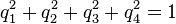
Inspection shows that the quaternion parametrization obeys the following constraint:

$q_1^2 + q_2^2 + q_3^2 + q_4^2 = 1$

The last term (in our definition) is often called the scalar term, which has its origin in quaternions when understood as the mathematical extension of the complex numbers, written as

$a + b i + c j + d k$ with $\{a, b, c, d\} \in \mathbb{R}$

and where $\scriptstyle \{i,\, j,\, k\}$ are the hypercomplex numbers satisfying

$\begin{array}{lclrlcl} i^2 &=& j^2 &=& k^2 &=& -1\\ ij &=& -ji &=& k&&\\ jk &=& -kj &=& i&&\\ ki &=& -ik &=& j&& \end{array}$

Quaternion multiplication is performed in the same manner as multiplication of complex numbers, except that the order of elements must be taken into account, since multiplication is not commutative. In matrix notation we can write quaternion multiplication as

$\tilde{\mathbf{q}}\otimes\mathbf{q} = \left[ {\begin{array}{rrrr} q_4 & q_3 & -q_2 & q_1\\ -q_3 & q_4 & q_1 & q_2\\ q_2 & -q_1 & q_4 & q_3\\ -q_1 & -q_2 & -q_3 & q_4 \end{array}} \right] \left[ {\begin{array}{c} \tilde{q}_1\\ \tilde{q}_2\\ \tilde{q}_3\\ \tilde{q}_4 \end{array}} \right] = \left[ {\begin{array}{rrrr} \tilde{q}_4 & -\tilde{q}_3 & \tilde{q}_2 & \tilde{q}_1\\ \tilde{q}_3 & \tilde{q}_4 & -\tilde{q}_1 & \tilde{q}_2\\ -\tilde{q}_2 & \tilde{q}_1 & \tilde{q}_4 & \tilde{q}_3\\ -\tilde{q}_1 & -\tilde{q}_2 & -\tilde{q}_3 & \tilde{q}_4 \end{array}} \right] \left[ {\begin{array}{c} q_1\\ q_2\\ q_3\\ q_4 \end{array}} \right]$

Combining two consecutive quaternion rotations is therefore just as simple as using the rotation matrix. Remember that two successive rotation matrices, $\scriptstyle \mathbf{A}_1$ followed by $\scriptstyle \mathbf{A}_2$ , are combined as follows:

$\mathbf{A}_3 = \mathbf{A}_2\mathbf{A}_1$

We can represent this with quaternion parameters in a similarly concise way:

$\mathbf{q}_3 = \mathbf{q}_2 \otimes \mathbf{q}_1$

Quaternions are a very popular parametrization due to the following properties:

More compact than the matrix representation and less susceptible to round-off errors
The quaternion elements vary continuously over the unit sphere in $\scriptstyle \mathbb{R}^4$ , (denoted by $\scriptstyle S^3$ ) as the orientation changes, avoiding discontinuous jumps (inherent to three-dimensional parameterizations)
Expression of the rotation matrix in terms of quaternion parameters involves no trigonometric functions
It is simple to combine two individual rotations represented as quaternions using a quaternion product

Like rotation matrices, quaternions must sometimes be re-normalized due to rounding errors, to make sure that they correspond to valid rotations. The computational cost of re-normalizing a quaternion, however, is much less than for normalizing a 3 × 3 matrix.

Rodrigues parameters

Main article: Euler–Rodrigues parameters

Cayley–Klein parameters

This section requires expansion. (September 2013)

See definition at Wolfram Mathworld.

Higher dimensional analogues

Conversion formulae between formalisms

Rotation matrix ↔ Euler angles

The Euler angles $\scriptstyle (\phi,\, \theta,\, \psi)$ can be extracted from the rotation matrix $\scriptstyle \mathbf{A}$ by inspecting the rotation matrix in analytical form.
Using the x-convention, the 3-1-3 Euler angles $\scriptstyle \phi$ , $\scriptstyle \theta$ and $\scriptstyle \psi$ (around the $\scriptstyle Z$ , $\scriptstyle X$ and again the $\scriptstyle Z$ -axis) can be obtained as follows:

$\begin{align} \phi &= \operatorname{arctan2}(A_{31}, A_{32})\\ \theta &= \arccos(A_{33})\\ \psi &= -\operatorname{arctan2}(A_{13}, A_{23}) \end{align}$

Note that $\scriptstyle \operatorname{arctan2}(a,\, b)$ is equivalent to $\scriptstyle \arctan(a/b)$ where it also takes into account the quadrant that the point $\scriptstyle (a,\, b)$ is in; see atan2.
When implementing the conversion, one has to take into account several situations:^[2]

There are generally two solutions in (−π, π]³ interval. The above formula works only when $\theta$ is from the interval [0, π)³.
For special case $\scriptstyle A_{33} \;=\; 0$ , $\scriptstyle \phi,\, \psi$ shall be derived from $\scriptstyle A_{11},\, A_{12}$ .
There is infinitely many but countably many solutions outside of interval (−π, π]³.
Whether all mathematical solutions apply for given application depends on the situation.

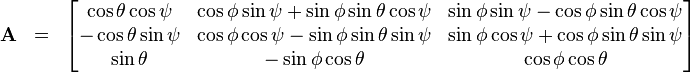
The rotation matrix $\scriptstyle \mathbf{A}$ is generated from the Euler angles by multiplying the three matrices generated by rotations about the axes.

$\mathbf{A} = \mathbf{A}_3\mathbf{A}_2\mathbf{A}_1 = \mathbf{A}_Z\mathbf{A}_Y\mathbf{A}_X$

The axes of the rotation depend on the specific convention being used. For the x-convention the rotations are about the $\scriptstyle X$ , $\scriptstyle Y$ and $\scriptstyle Z$ axes with angles $\scriptstyle \phi$ , $\scriptstyle \theta$ and $\scriptstyle \psi$ , the individual matrices are as follows:

$\begin{align} \mathbf{A}_X &= \left[\begin{array}{ccc} 1 & 0 & 0\\ 0 & \cos\phi & \sin\phi\\ 0 & -\sin\phi & \cos\phi \end{array} \right]\\ \mathbf{A}_Y &= \left[\begin{array}{ccc} \cos\theta & 0 & -\sin\theta\\ 0 & 1 & 0\\ \sin\theta & 0 & \cos\theta \end{array} \right]\\ \mathbf{A}_Z &= \left[\begin{array}{ccc} \cos\psi & \sin\psi & 0\\ -\sin\psi & \cos\psi & 0\\ 0 & 0 & 1 \end{array} \right] \end{align}$

This yields

$\begin{array}{lcl} \mathbf{A} &=& \begin{bmatrix} \cos\theta \cos\psi & \cos\phi \sin\psi + \sin\phi \sin\theta \cos\psi & \sin\phi \sin\psi - \cos\phi \sin\theta \cos\psi \\ -\cos\theta \sin\psi & \cos\phi \cos\psi - \sin\phi \sin\theta \sin\psi & \sin\phi \cos\psi + \cos\phi \sin\theta \sin\psi \\ \sin\theta & -\sin\phi \cos\theta & \cos\phi \cos\theta \\ \end{bmatrix} \end{array}$

Note: This is valid for a right-hand system, which is the convention used in almost all engineering and physics disciplines.

Rotation matrix ↔ Euler axis/angle

It has been suggested that Rotation matrix#Conversion from and to axis-angle be merged into this section. (Discuss) Proposed since September 2013.

If the Euler angle $\scriptstyle \theta$ is not a multiple of $\scriptstyle \pi$ , the Euler axis $\scriptstyle \hat{\mathbf{e}} \;=\; [e_1\ e_2\ e_3]^\mathrm{T}$ and angle $\scriptstyle \theta$ can be computed from the elements of the rotation matrix $\scriptstyle \mathbf{A}$ as follows:

$\begin{align} \theta &= \arccos\left(\frac{1}{2}[A_{11}+A_{22}+A_{33}-1]\right)\\ e_1 &= \frac{A_{32}-A_{23}}{2\sin\theta}\\ e_2 &= \frac{A_{13}-A_{31}}{2\sin\theta}\\ e_3 &= \frac{A_{21}-A_{12}}{2\sin\theta} \end{align}$

Alternatively, the following method can be used:
Eigen-decomposition of the rotation matrix yields the eigenvalues 1, and $\scriptstyle \cos\theta \pm i\sin\theta$ . The Euler axis is the eigenvector corresponding to the eigenvalue of 1, and the $\scriptstyle \theta$ can be computed from the remaining eigenvalues.
The Euler axis can be also found using Singular Value Decomposition since it is the normalized vector spanning the null-space of the matrix $\scriptstyle I \,-\, A$ .
To convert the other way the rotation matrix corresponding to an Euler axis $\scriptstyle \hat{\mathbf{e}} \;=\; [e_1\ e_2\ e_3]^\mathrm{T}$ and angle $\scriptstyle \theta$ can be computed according to the Rodrigues' rotation formula (with appropriate modification) as follows:

$\mathbf{A} = \mathbf{I}_3\cos\theta + (1-\cos\theta)\hat{\mathbf{e}}\hat{\mathbf{e}}^\mathrm{T} + [\hat{\mathbf{e}}]_{\times} \sin\theta$

with $\scriptstyle \mathbf{I}_3$ the 3 × 3 identity matrix, and

$[\hat{\mathbf{e}}]_{\times} = \left[\begin{array}{ccc} 0 & -e_3 & e_2\\ e_3 & 0 & -e_1\\ -e_2 & e_1 & 0 \end{array} \right]$

is the cross-product matrix.

Rotation matrix ↔ quaternion

When computing a quaternion from the rotation matrix there is a sign ambiguity, since $\scriptstyle \mathbf{q}$ and $\scriptstyle -\mathbf{q}$ represent the same rotation.
One way of computing the quaternion $\scriptstyle \mathbf{q} \;=\; [q_1\ q_2\ q_3\ q_4]^\mathrm{T}$ from the rotation matrix $\scriptstyle \mathbf{A}$ is as follows:

$\begin{align} q_4 &= \frac{1}{2}\sqrt{1+A_{11}+A_{22}+A_{33}}\\ q_1 &= \frac{1}{4q_4}(A_{32}- A_{23})\\ q_2 &= \frac{1}{4q_4}(A_{13}- A_{31})\\ q_3 &= \frac{1}{4q_4}(A_{21}- A_{12}) \end{align}$

There are three other mathematically equivalent ways to compute $\scriptstyle \mathbf{q}$ . Numerical inaccuracy can be reduced by avoiding situations in which the denominator is close to zero. One of the other three methods looks as follows:^[3]

$\begin{align} q_1 &= \frac{1}{2}\sqrt{1 + A_{11} - A_{22} - A_{33}}\\ q_2 &= \frac{1}{4q_1}(A_{12} + A_{21})\\ q_3 &= \frac{1}{4q_1}(A_{13} + A_{31})\\ q_4 &= \frac{1}{4q_1}(A_{32} - A_{23}) \end{align}$

The rotation matrix corresponding to the quaternion $\scriptstyle \mathbf{q} \;=\; [q_1\ q_2\ q_3\ q_4]^\mathrm{T}$ can be computed as follows:

$\mathbf{A} = (q_4^2 - \check{\mathbf{q}}^\mathrm{T}\check{\mathbf{q}})\mathbf{I}_3 + 2\check{\mathbf{q}}\check{\mathbf{q}}^\mathrm{T} + 2q_4\mathbf{\mathcal{Q}}$

with $\scriptstyle \mathbf{I}_3$ the 3 × 3 identity matrix, and

$\check{\mathbf{q}} = \left[\begin{array}{c} q_1\\q_2\\q_3\end{array} \right],\ \ \ \mathbf{\mathcal{Q}} = \left[\begin{array}{ccc} 0 & -q_3 & q_2\\ q_3 & 0 & -q_1\\ -q_2 & q_1 & 0 \end{array} \right]$

which gives

$\mathbf{A} = \left[\begin{array}{ccc} 1 - 2q_2^2 - 2q_3^2 & 2(q_1q_2 - q_3q_4) & 2(q_1q_3 + q_2q_4)\\ 2(q_1q_2 + q_3q_4) & 1 - 2q_1^2- 2 q_3^2 & 2(q_2q_3 - q_1q_4)\\ 2(q_1q_3 - q_2q_4) & 2(q_1q_4 + q_2q_3) & 1 - 2q_1^2 - 2q_2^2 \end{array} \right]$

or equivalently

$\mathbf{A} = \left[\begin{array}{ccc} -1 + 2q_1^2 + 2q_4^2 & 2(q_1q_2 - q_3q_4) & 2(q_1q_3 + q_2q_4)\\ 2(q_1q_2 + q_3q_4) & -1 + 2q_2^2 + 2q_4^2 & 2(q_2q_3 - q_1q_4)\\ 2(q_1q_3 - q_2q_4) & 2(q_1q_4 + q_2q_3) & -1 + 2q_3^2 + 2q_4^2 \end{array} \right]$

Euler angles ↔ quaternion

Main article: Conversion between quaternions and Euler angles

We will consider the x-convention 3-1-3 Euler Angles for the following algorithm. The terms of the algorithm depend on the convention used.
We can compute the quaternion $\scriptstyle \mathbf{q} = [q_1\ q_2\ q_3\ q_4]^\mathrm{T}$ from the Euler angles $\scriptstyle (\phi,\, \theta,\, \psi)$ as follows:

$\begin{align} q_1 &= \cos\left(\frac{\phi - \psi}{2}\right)\sin\left(\frac{\theta}{2}\right)\\ q_2 &= \sin\left(\frac{\phi - \psi}{2}\right)\sin\left(\frac{\theta}{2}\right)\\ q_3 &= \sin\left(\frac{\phi + \psi}{2}\right)\cos\left(\frac{\theta}{2}\right)\\ q_4 &= \cos\left(\frac{\phi + \psi}{2}\right)\cos\left(\frac{\theta}{2}\right) \end{align}$

Given the rotation quaternion $\scriptstyle \mathbf{q} = [q_1\ q_2\ q_3\ q_4]^\mathrm{T}$ , the x-convention 3-1-3 Euler angles $\scriptstyle (\phi,\, \theta,\, \psi)$ can be computed by

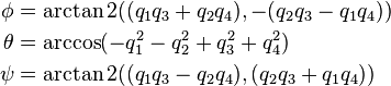
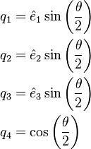
$\begin{align} \phi &= \arctan2((q_1q_3 + q_2q_4), -(q_2q_3 - q_1q_4))\\ \theta &= \arccos(-q_1^2 - q_2^2 + q_3^2+q_4^2)\\ \psi &= \arctan2((q_1q_3 - q_2q_4), (q_2q_3 + q_1q_4)) \end{align}$

Euler axis/angle ↔ quaternion

Given the Euler axis $\scriptstyle \hat{\mathbf{e}}$ and angle $\scriptstyle \theta$ , the quaternion

$\mathbf{q} = [q_1\ q_2\ q_3\ q_4]^\mathrm{T}$

can be computed by

$\begin{align} q_1 &= \hat{e}_1\sin\left(\frac{\theta}{2}\right) \\ q_2 &= \hat{e}_2\sin\left(\frac{\theta}{2}\right) \\ q_3 &= \hat{e}_3\sin\left(\frac{\theta}{2}\right) \\ q_4 &= \cos\left(\frac{\theta}{2}\right) \end{align}$

Given the rotation quaternion $\scriptstyle \mathbf{q} \;=\; [q_1\ q_2\ q_3\ q_4]^\mathrm{T}$ , define $\scriptstyle \check{\mathbf{q}} \;=\; [q_1\ q_2\ q_3]^\mathrm{T}$ . Then the Euler axis $\scriptstyle \hat{\mathbf{e}}$ and angle $\scriptstyle \theta$ can be computed by

$\begin{align} \hat{\mathbf{e}} &= \frac{\check{\mathbf{q}}}{\|\check{\mathbf{q}}\|} \\ \theta &= 2\arccos(q_4) \end{align}$

Conversion formulae for derivatives

Rotation matrix ↔ angular velocities

The angular velocity vector $\scriptstyle \mathbf{\omega} \;=\; (\omega_x,\, \omega_y,\, \omega_z)$ can be extracted from the derivative of the rotation matrix $\scriptstyle \frac{d\mathbf{A}}{dt}$ by the following relation:

$[\mathbf{\omega}]_\times = \left[\begin{array}{ccc} 0 & -\omega_z & \omega_y \\ \omega_z & 0 & -\omega_x \\ -\omega_y & \omega_x & 0 \end{array} \right] = \frac{d\mathbf{A}}{dt}\mathbf{A}^\mathrm{T}$

The derivation is adapted from ^[4] as follows:
For any vector $\scriptstyle r_0$ consider $\scriptstyle r(t) \;=\; \mathbf{A}(t) r_0$ and differentiate it:

$\frac{dr}{dt} = \frac{d\mathbf{A}}{dt} r_0 = \frac{d\mathbf{A}}{dt} \mathbf{A}^\mathrm{T}(t) r(t)$

The derivative of a vector is the linear velocity of its tip. Since A is a rotation matrix, by definition the length of $\scriptstyle r(t)$ is always equal to the length of $\scriptstyle r_0$ , and hence it does not change with time. Thus, when $\scriptstyle r(t)$ rotates, its tip moves along a circle, and the linear velocity of its tip is tangential to the circle; i.e., always perpendicular to $\scriptstyle r(t)$ . In this specific case, the relationship between the linear velocity vector and the angular velocity vector is

$\frac{dr}{dt} = \mathbf{\omega}(t)\times r(t) = [\mathbf{\omega}]_\times r(t)$ (see circular motion and Cross product).

By the transitivity of the above mentioned equations,

$\frac{d\mathbf{A}}{dt} \mathbf{A}^\mathrm{T}(t) r(t) = [\mathbf{\omega}]_\times r(t)$

which implies (Q.E.D.),

$\frac{d\mathbf{A}}{dt} \mathbf{A}^\mathrm{T}(t) = [\mathbf{\omega}]_\times$

Quaternion ↔ angular velocities

The angular velocity vector $\scriptstyle \mathbf{\omega} \;=\; (\omega_x,\, \omega_y,\, \omega_z)$ can be obtained from the derivative of the quaternion $\scriptstyle \frac{d\mathbf{q}}{dt}$ as follows:^[5]

$\left[ {\begin{array}{c} 0 \\ \omega_x \\ \omega_y \\ \omega_z \end{array}} \right] = 2 \frac{d\mathbf{q}}{dt} \otimes \tilde{\mathbf{q}}$

where $\tilde{\mathbf{q}}$ is the inverse of $\mathbf{q}$ .
Conversely, the derivative of the quaternion is

$\frac{d\mathbf{q}}{dt} = \frac{1}{2}\left[ {\begin{array}{c} 0 \\ \omega_x\\ \omega_y\\ \omega_z \end{array}} \right] \otimes \mathbf{q}$

Rotors in a geometric algebra

It has been suggested that this section be merged into Geometric algebra#Rotations. (Discuss) Proposed since September 2013.

The formalism of geometric algebra (GA) provides an extension and interpretation of the quaternion method. Central to GA is the geometric product of vectors, an extension of the traditional inner and cross products, given by

$ab = a \cdot b + a \wedge b$

where the symbol $\scriptstyle \wedge$ denotes the outer product. This product of vectors $\scriptstyle a,\, b$ produces two terms: a scalar part from the inner product and a bivector part from the outer product. This bivector describes the plane perpendicular to what the cross product of the vectors would return.
Bivectors in GA have some unusual properties compared to vectors. Under the geometric product, bivectors have negative square: the bivector $\scriptstyle \hat x \hat y$ describes the $\scriptstyle xy$ -plane. Its square is $\scriptstyle (\hat x \hat y)^2 \;=\; \hat x \hat y \hat x \hat y$ . Because the unit basis vectors are orthogonal to each other, the geometric product reduces to the antisymmetric outer product – $\scriptstyle \hat x$ and $\scriptstyle \hat y$ can be swapped freely at the cost of a factor of −1. The square reduces to $\scriptstyle -\hat x \hat x \hat y \hat y \;=\; -1$ since the basis vectors themselves square to +1.
This result holds generally for all bivectors, and as a result the bivector plays a role similar to the imaginary unit. Geometric algebra uses bivectors in its analogue to the quaternion, the rotor, given by $\scriptstyle R \;=\; \exp\left(\frac{-\hat B\theta}{2}\right) \;=\; \cos \frac{\theta}{2} \,-\, \hat B \sin \frac{\theta}{2}$ , where $\scriptstyle \hat B$ is a unit bivector that describes the plane of rotation. Because $\scriptstyle \hat B$ squares to −1, the power series expansion of $\scriptstyle R$ generates the trigonometric functions. The rotation formula that maps a vector $\scriptstyle a$ to a rotated vector $\scriptstyle b$ is then

$b = R a R^\dagger$

where $\scriptstyle R^\dagger \;=\; \exp\left(\frac{1}{2}\hat B \theta\right) \;=\; \cos \frac{1}{2}\theta \,+\, \hat B \sin \frac{1}{2}\theta$ is the reverse of $\scriptstyle R$ (reversing the order of the vectors in $\scriptstyle B$ is equivalent to changing its sign).
Example. A rotation about the axis $\scriptstyle \hat v \;=\; \frac{1}{\sqrt{3}}(\hat x \,+\, \hat y \,+\, \hat z)$ can be accomplished by converting $\scriptstyle \hat v$ to its dual bivector, $\scriptstyle \hat B \;=\; \hat x \hat y \hat z \hat v \;=\; i \hat v$ , where $\scriptstyle i \;=\; \hat x \hat y \hat z$ is the unit volume element, the only trivector (pseudoscalar) in three-dimensional space. The result is $\scriptstyle \hat B \;=\; \frac{1}{\sqrt{3}}(\hat y \hat z \,+\, \hat z \hat x \,+\, \hat x \hat y)$ . In three-dimensional space, however, it is often simpler to leave the expression for $\scriptstyle \hat B \;=\; i \hat v$ , using the fact that $\scriptstyle i$ commutes with all objects in 3D and also squares to −1. A rotation of the $\scriptstyle \hat x$ vector in this plane by an angle $\scriptstyle \theta$ is then

$\hat x' = R \hat x R^\dagger = e^{-i\hat v \frac{\theta}{2}} \hat x e^{i \hat v \frac{\theta}{2}} = \hat x \cos^2 \frac{\theta}{2} + i (\hat x \hat v - \hat v \hat x) \cos \frac{\theta}{2} \sin \frac{\theta}{2} + \hat v \hat x \hat v \sin^2 \frac{\theta}{2}$

Recognizing that $\scriptstyle i (\hat x \hat v \,-\, \hat v \hat x) \;=\; 2i (\hat x \,\wedge\, \hat v)$ and that $\scriptstyle -\hat v \hat x \hat v$ is the reflection of $\scriptstyle \hat x$ about the plane perpendicular to $\scriptstyle \hat v$ gives a geometric interpretation to the rotation operation: the rotation preserves the components that are parallel to $\scriptstyle \hat v$ and changes only those that are perpendicular. The terms are then computed:

$\begin{align} \hat v \hat x \hat v &= \frac{1}{3} (-\hat x + 2 \hat y + 2 \hat z) \\ 2i \hat x \wedge \hat v &= 2i \frac{1}{\sqrt{3}} (\hat x \hat y + \hat x \hat z) = \frac{2}{\sqrt{3}} (\hat y - \hat z) \end{align}$

The result of the rotation is then

$\hat x' = \hat x \left(\cos^2 \frac{\theta}{2} - \frac{1}{3} \sin^2 \frac{\theta}{2}\right) + \frac{2}{3} \hat y \sin \frac{\theta}{2} \left(\sin \frac{\theta}{2} + \sqrt{3} \cos \frac{\theta}{2}\right) + \frac{2}{3} \hat z \sin \frac{\theta}{2} \left(\sin \frac{\theta}{2} - \sqrt{3} \cos \frac{\theta}{2}\right)$

A simple check on this result is the angle $\scriptstyle \theta \;=\; \frac{2}{3}\pi$ . Such a rotation should map the $\scriptstyle \hat x$ to $\scriptstyle \hat y$ . Indeed, the rotation reduces to

$\begin{align} \hat x' &= \hat x\left(\frac{1}{4} - \frac{1}{3} \frac{3}{4}\right) + \frac{2}{3} \hat y \frac{\sqrt{3}}{2} \left(\frac{\sqrt{3}}{2} + \sqrt{3}\frac{1}{2}\right) + \frac{2}{3} \hat z \frac{\sqrt{3}}{2} \left(\frac{\sqrt{3}}{2} - \sqrt{3}\frac{1}{2}\right) \\ &= 0 \hat x + \hat y + 0 \hat z = \hat y \end{align}$

exactly as expected. This rotation formula is valid not only for vectors but for any multivector. In addition, when Euler angles are used, the complexity of the operation is much reduced. Compounded rotations come from multiplying the rotors, so the total rotor from Euler angles is

$R = R_{\gamma'} R_{\beta'} R_\alpha = \exp\left(\frac{-i \hat z' \gamma}{2}\right) \exp\left(\frac{-i \hat x' \beta}{2}\right) \exp\left(\frac{-i \hat z \alpha}{2}\right)$

but $\scriptstyle \hat x' \;=\; R_\alpha \hat x R_\alpha^\dagger$ and $\scriptstyle \hat z' \;=\; R_{\beta'} \hat z R_{\beta'}^\dagger$ . These rotors come back out of the exponentials like so:

$R_{\beta'} = \cos \frac{\beta}{2} - i R_\alpha \hat x R_\alpha^\dagger \sin \frac{\beta}{2} = R_\alpha R_\beta R_\alpha^\dagger$

where $\scriptstyle R_\beta$ refers to rotation in the original coordinates. Similarly for the $\scriptstyle \gamma$ rotation, $\scriptstyle R_{\gamma'} \;=\; R_{\beta'} R_\gamma R_{\beta'}^\dagger \;=\; R_\alpha R_\beta R_\alpha^\dagger R_\gamma R_\alpha R_\beta^\dagger R_\alpha^\dagger$ . Noting that $\scriptstyle R_\gamma$ and $\scriptstyle R_\alpha$ commute (rotations in the same plane must commute), and the total rotor becomes

$R = R_\alpha R_\beta R_\gamma$

Thus, the compounded rotations of Euler angles become a series of equivalent rotations in the original fixed frame.
While rotors in geometric algebra work almost identically to quaternions in three dimensions, the power of this formalism is its generality: this method is appropriate and valid in spaces with any number of dimensions. In 3D, rotations have three degrees of freedom, a degree for each linearly independent plane (bivector) the rotation can take place in. It has been known that pairs of quaternions can be used to generate rotations in 4D, yielding six degrees of freedom, and the geometric algebra approach verifies this result: in 4D, there are six linearly independent bivectors that can be used as the generators of rotations.

Politeknik Tuanku Sultanah Bahiyah PTSB kulim, belajar baca motivasi kerja sekolah dan puisi

Monday, 2 December 2013

Attitude representations